
Activity – Excel 1: Getting started
![]() To navigate this press book use the menu from the top left corner.
To navigate this press book use the menu from the top left corner.

Spreadsheets with Excel
In week 2, you learned how to make a table to present information in Word. Whilst this is an important skill, you must also make tables in MS Excel. A table in excel also has columns and rows, however, the document created is called a worksheet and has the advantage that it can perform many calculations, saving you lots of time.
Microsoft (MS) Excel is a common spreadsheet application that enables users to organise, analyse, manage, and share data easily. Excel also enables users to create charts to represent the data in the worksheets visually.
An Excel document is called a workbook. Each workbook consists of one or multiple pages, known as sheets or worksheets. When you consider the ability to perform calculations and create graphs, you have a powerful tool that you can use to analyse and present your data.
Work through the Excel activities in this Pressbook to develop your understanding of Excel. This knowledge will be required to help you complete content for your assignment 4. You are also required to submit certain activities. Please check the instructions for assignments 3 and 4 for further information.
Activity – Excel 1
1. Click the Windows icon at the bottom of your screen.
2. Click Excel to launch Microsoft Excel.
3. Click Blank Workbook to create a new presentation document.
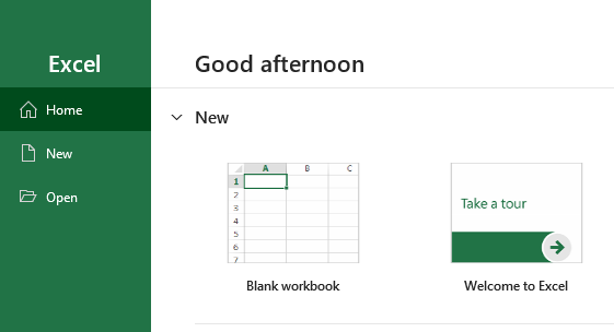
A new workbook is created.
4. Have a close look at the screenshot below to familiarize yourself with the Excel working area
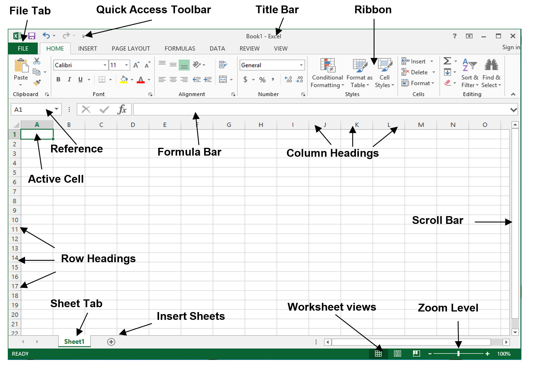
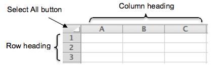
A worksheet is divided into a grid of columns and rows. The intersection of a column and row is a cell. Every column is labelled with a letter (shown in its heading) and every row with a number. The combination of a column letter and row number uniquely identifies each cell, such as B3 or D15. This combination is known as a cell reference (cell address).
For example, the cell reference of the active cell in the above screenshot is A1, which is the intersection of Column A and Row 1.
An active cell is a single cell with a thick green rectangle border. It is the cell that receives input from the keyboard.
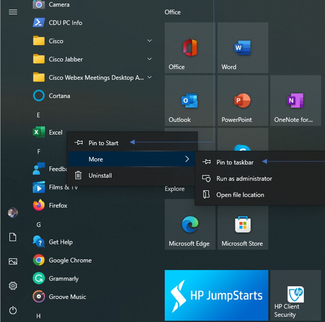
 If you use Excel often, you can pin the application to the Start menu. From the All apps list in the Start menu, right-click the app name (Excel), and choose Pin to Start.
You can also choose More and then Pin to the taskbar to allow you to click the icon in the Windows taskbar at the bottom of the screen to start Excel.
Quick Access Toolbar
The Quick Access Toolbar gives you fast and easy access to the tools you use most often in Excel. It appears on the left side of the title bar, above the ribbon. You can add and remove commands to and from the toolbar so that it contains only those commands you use most frequently.
Customizing the Quick Access Toolbar
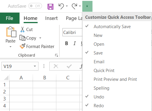
Click the drop-down arrow on the right side of the Quick Access Toolbar, From the drop-down list, select Open. The Open icon is added to the Quick Access Toolbar. Click the down arrow again and select Quick Print from the drop-down list.
By default, the Quick Access Toolbar contains the Save, Undo, and Redo commands. As you work in Excel, customize the Quick Access Toolbar so that it contains the commands you use most often. Do not, however, remove the Undo and Redo commands. These commands are not available on the ribbon’s command tabs.
To add commands to the Quick Access Toolbar that do not appear in the drop-down list, click More Commands on the drop-down list. The Excel Options dialog box opens. You can also right-click the Quick Access Toolbar or any ribbon tab and select Customize Quick Access Toolbar to open the Excel Options dialog box.
Entering Data
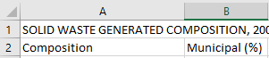
- Click in cell A1 to make the cell active
- Type SOLID WASTE GENERATED COMPOSITION, 2002–03, and press Enter key.
 Note that the text you typed appears in two locations – inside cell A1 and in the Formula Bar.
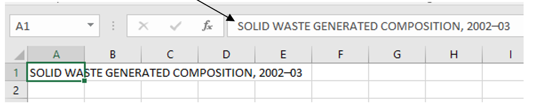
3. Click in cell A2, Type Composition, and press the Tab key.
 You may have noticed that after entering text in a cell,
- pressing Enter key moves the active cell down a cell
- pressing the Tab key moves the active cell to the adjacent cell to the right.
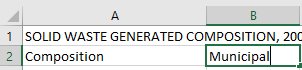
4. Type Municipal and press the Tab key.
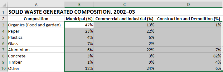
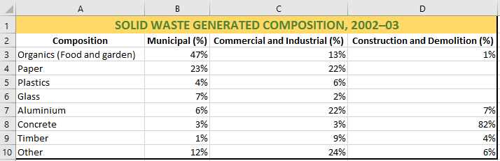
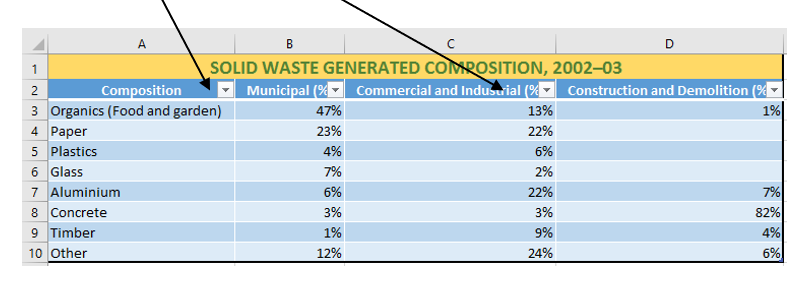
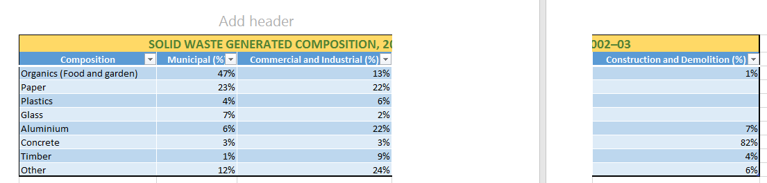
Complete the table by entering the data below. The data shown below indicates solid waste generated composition in Australia between the years 2002 and 2003. Note that the blank cells represent nil or have been rounded to zero.
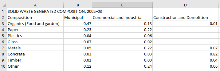
Source: Australian Bureau of Statistics, 2006, Australia’s Environment Issues and Trends, Catalogue No: 4613.0
5. Click the File tab
6. Click Save As and then Browse.
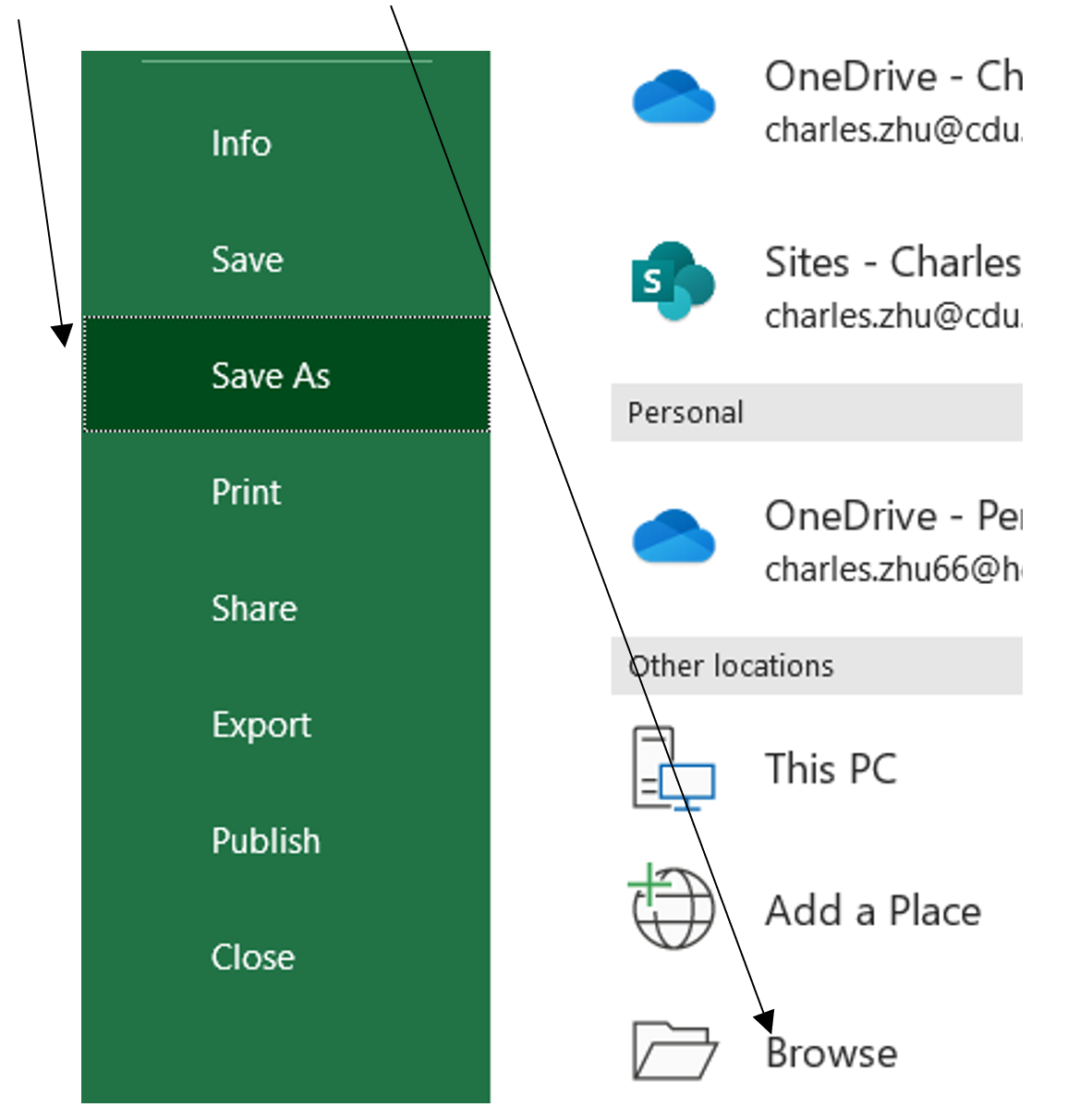
7. Click Documents and then name the spreadsheet Your Name TEP021 Excel 1.xlsx
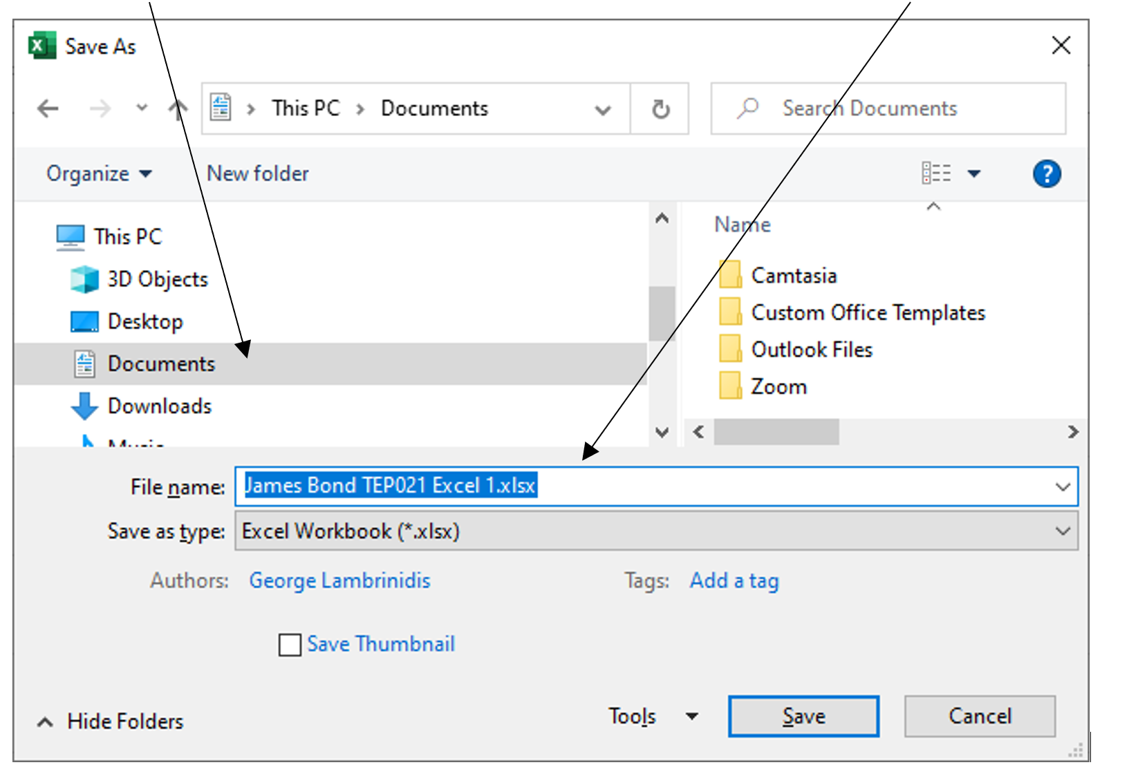
8. Click Save. Your Spreadsheet is saved in the Documents folder on your computer.
Editing Data
You can edit data (text or numbers in a cell) either directly in the cell or using the Formula Bar.
Editing data directly in a cell
-
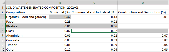
- Click once in the cell containing the word Metals to make it active.
- Type Aluminium and press Enter key to replace the content in the cell.
Typing in an active cell replaces ALL contents in the cell.
3. Double-click the cell containing Municipal.
4. Move the flashing cursor to the end of the word using arrow keys.
5. Enter a space followed by (%) and then press Enter.
Double-clicking a cell puts the inserting cursor into the cell and enables direct editing in the cell.
6. Add a space followed by (%) to both the column C and D headings.
Editing data in Formula Bar
The content of the active cell can also be edited in the Formula Bar.
7. Click once in cell B7, containing the value 0.05 to make it active.
8. Click in the Formula Bar to activate Formula Bar editing mode. The flashing cursor is displayed in the Formula Bar.
9. Delete 0.05 by pressing the backspace or delete key and then type 0.06 as shown below:
![]()
10. Press the Enter key or click the tick to accept the editing. If you want to cancel the editing, click the cross.
11. Save your work and keep the document open.
Selecting Cells
To work with a single cell, you simply click it or use the arrow keys on the keyboard to move the active cell to it. When you need to edit multiple cells at once, you select the cells using the mouse or keyboard.
Excel calls a selection of cells a range. A range can consist of either a rectangle of contiguous cells that are all next to each other or a range of dispersed cells that aren’t next to each other, called non-contiguous.
Selecting Contiguous Cells
You can select a range of contiguous cells in any of the following three ways which you can practice:
12. Click and drag. Click the first cell in a range and hold down the mouse button, then drag across to select all the others.
For example, click cell B3 and hold down the mouse button, then drag to cell D10, you select a range of four columns wide and six rows deep. 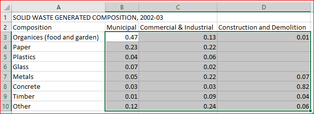
Excel uses the notation B3:D10 to describe this range—the starting cell address, a colon, and then the ending cell address.
To deselect a range you’ve selected, click anywhere outside the range.
- Click and then Shift + click. Click the first cell in the range, then hold down the Shift key and click the last cell. Excel selects all the cells in between. This technique tends to be the easiest to use when the first cell and last cell are widely separated.
- Hold down the Shift key and select with the arrow keys. Make the first cell of the range active, then hold down the Shift key and use the arrow keys to extend the selection for the rest of the range. This method is good if you prefer using the keyboard to the mouse.
Selecting Non-contiguous Cells
To select a range of non-contiguous cells:
- Select the first range of contiguous cells, and then
- Hold down the Ctrl key and select the second range of (third, fourth, and so on…) contiguous cells.
Excel uses commas to separate the individual cells in this type of range.
For example, the range B3, A5:C5, C6:D6 consists of one individual cell (B3) and two ranges of contiguous cells (A5 through C5 and C6 through D6) as shown in the example below:
Selecting the Entire Row or Column
You can quickly select a row by clicking its row heading (the Number) or pressing Shift + Spacebar when the active cell is in that row.
Likewise, you can select a column by clicking its column heading (the Letter) or pressing Ctrl + Spacebar.
Selecting the Entire worksheet
To select all the cells in the active worksheet,
Click the Select All button (where the row headings and column headings meet).
OR
Press Ctrl + A
Deleting the Content of a Cell or a Range
To delete the content of a single cell, click the cell and press the Backspace or Delete key.
To delete the contents of a range, select the cell range and press the Delete key. Pressing the Backspace key will delete the content in the first cell only.
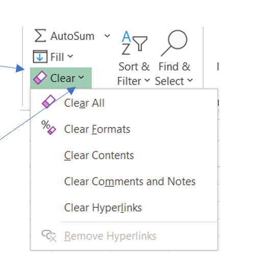
You can also use the Clear command (from the Home ribbon) to remove the contents or/and formats of the selected cell(s)
Simply clicking the Clear icon clears all the content from the cell/s or range, including formats, contents, and comments. However, you can be specific and choose to clear formats only, or contents only by clicking the drop-down arrow and selecting an option.
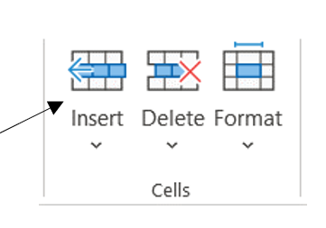
Inserting Columns and Rows
Select the column/row where the new column/row should appear and then click the Insert command icon on the Home ribbon.1.
The new column will push the selected column to right. The new row will push the selected row down.
1. Select the entire Column D, which is the column of Construction and Demolition (%).
2. Click Insert. The Construction and Demolition (%) column D becomes column E.
3. Select the entire Row 2
4. Click Insert.
Deleting Columns and Rows
1. Select the entire Column D, which is blank.
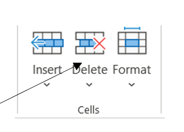
2. Click Delete.
3. Select the entire Row 2, which is blank.
4. Click Delete.
Changing Column Width and Row Height
Do one of the following to adjust the column width or row height:
Move the mouse pointer onto the grid between the column/row headings.
When the mouse pointer changes to  , hold the mouse button and drag left or right to adjust column width.
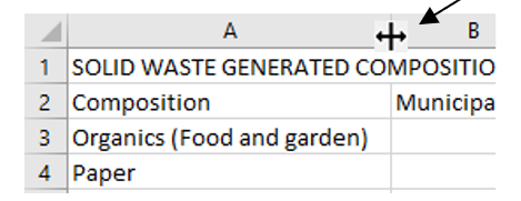
When the mouse pointer changes to![]() , hold the mouse button and drag it up or down to adjust row height.
, hold the mouse button and drag it up or down to adjust row height.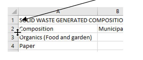
Double-click the right edge of a column heading to automatically adjust the column width to fit the longest text string in the column.
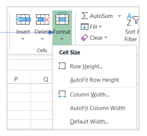
Click Format and select AutoFit Row Height/AutoFit Column Width to automatically adjust the height or width.
OR
Click Format and then Row Height…/Column Width… to assign a numerical value for the height or width.
Formatting Data
In Excel, you can format cells in a wide variety of ways — from choosing how to display the borders and background to controlling how Excel displays the data you enter in the cell.
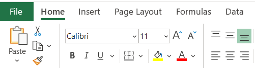
Formatting text
Excel offers a wide range of formatting that you can apply to text. You can specify a font, colour, styles (such as boldface or italic), and an alignment to selected cells.
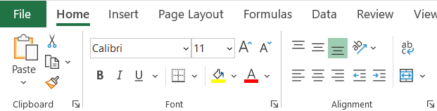
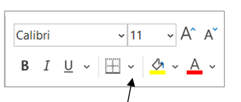
The familiar icons you used in Word are used in the same way to format text in Excel.
- Click cell A1 to make it active.
- Change the font size to 14 and make it Bold.
- Select cell range A2:D2 by clicking and dragging over from A2 to D2.
- Apply Center Text alignment and Bold (Note that Excel uses American English for “center” rather than “centre”).
Formatting Numbers
When you enter a number in a cell, Excel displays it according to the number formatting applied to that cell. For example, if you enter 42648 in a cell formatted with General formatting, Excel displays it as 42648.
If the cell has Currency formatting, Excel displays a value of $42,648.00. And if the cell has Date formatting, Excel displays a date of 5 October 2016.
In each case, the number stored in the cell remains the same – so if you change the cell’s formatting to a different type, Excel will display the data to reflect the format.
Select the range B3:D10 (cells from B3 to D10).
1. Click the drop-down arrow and select Percentage.
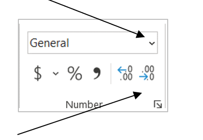
2. Click the Decrease Decimal icon twice. The decimals are hidden and only whole percentage values are displayed.
Merge cells
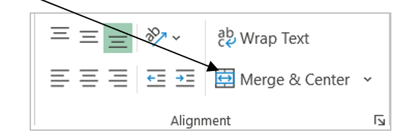
The table title SOLID WASTE GENERATED COMPOSITION, 2002–03 was entered and stored in cell A1. To centre the title above the table, use the Merge & Centre tool which will merge the cells A1:D1 into one cell.
-
- Select the cells A1:D1.
2. Click Merge & Center to merge the cells and the centre the text.
3. Save your work and keep your document open.
Adding cell borders and shading
A border is a line (or lines) at the edge of a cell. You can use borders to divide information on the sheet into logical regions. Shading is a colour or pattern used to fill selected cells.
- Ensure the heading A1:D1 remains highlighted.
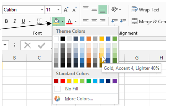
- Click the down arrow of the Fill Colour icon and choose Gold Accent 4 Lighter 40%.
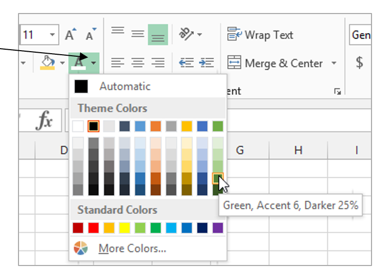
- Click the down arrow of the Font Colour icon and choose Green, Accent 6, Darker 25%.
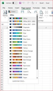
Note: If you cannot see the Gold, Accent 4, Lighter 40%, you may need to update the colour scheme. To do this, click on Page Layout then Colours, and select Office 2012-2022 as shown below:
4. Select the range A1:D10
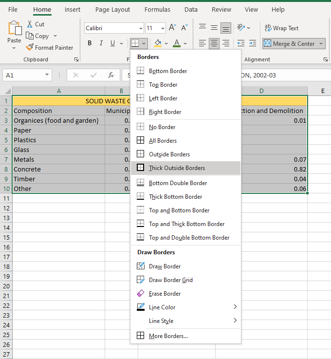
5. Click on the down arrow of the Border icon and select Thick Outside Borders as shown below:
Your Excel table should now appear with a golden colour header with green font and a solid border around it.
6. Save your work and keep your document open.
Applying Table Styles
An Excel table is a rectangular display of data that is independent of the rest of the worksheet. That is, you can perform most actions within a table without affecting data elsewhere. A table has the following advantages over a normal worksheet range:
- You can sort the entire table by column without affecting data above or below the table.
- You can quickly format your data using the Table Styles.
- You can add or delete rows/columns without damaging the worksheet’s integrity.
- Select the range A2:D10.
 Do not include the table title when you apply Table Styles.
2. Click the Format as Table, Select a table style of your choice from the Table Styles gallery.
Click OK in the small Format as Table dialog box that pops up.
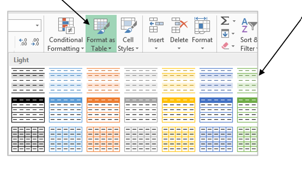
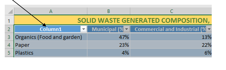
The Table Style formats the selected data range into a table with filters and sorting options (the arrow buttons) so that you can filter and sort the data in that table independently. A formatted table must have unique column headers (which can also be called Field Name).
If a column header is missing, Excel will add a header using the default value “Column1, Column2….”. Note: The original header “Composition” was deleted in the screenshot below, to demonstrate how Excel will add a “Column 1” automatically.
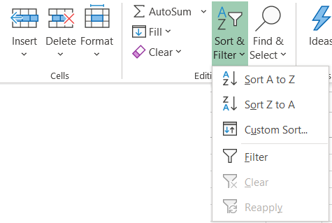
Hiding Filter Buttons
You can hide the filter buttons by turning the filter feature off. You can turn it on again if you need it later.
Click Filter to toggle on and off.
Changing the Spreadsheet Orientation
Sometimes a table or chart is too wide to fit into a portrait-oriented page and splits over two pages.

- Click the Page Layout button at the lower right corner of the Excel window to switch to Page Layout view.
You may notice that your Excel table splits over two pages.
One of the ways to fit a table or chart into one page is to change the page orientation to landscape.
2. Click the Page Layout tab.
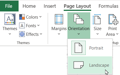
3. Click Orientation and select Landscape.
Headers and Footers
You can add headers, footers, or both to identify the pages. Excel gives each worksheet a separate header and footer, which you can fill with either pre-set text or custom text. Each header and footer area consists of a left section, a centre section, and a right section, so you can easily add several different pieces of information.
Adding Headers and Footers
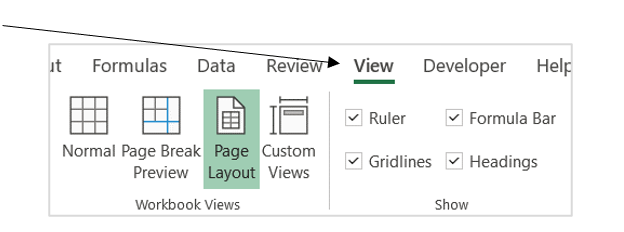
- Click the View tab and then Page Layout.
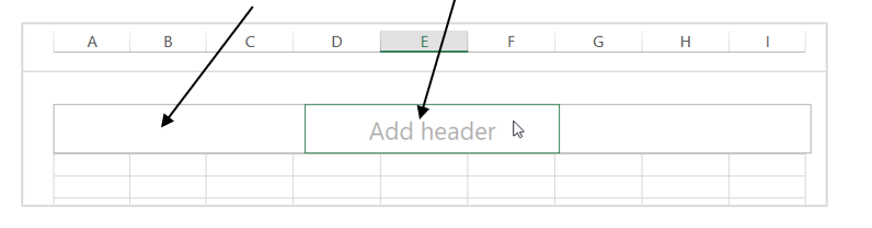
2. Move the mouse pointer over the words “Add header”, and the header area turns into three sections. Click in the left section.
3. Type your full name and student number then press the Tab key twice to move to the right section.
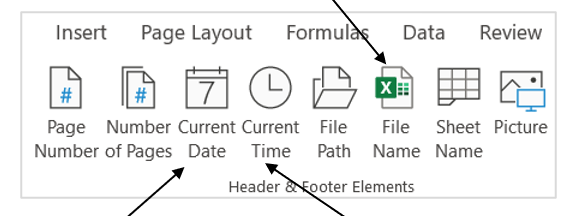
4. On the Header & Footer tab, click Page Number.
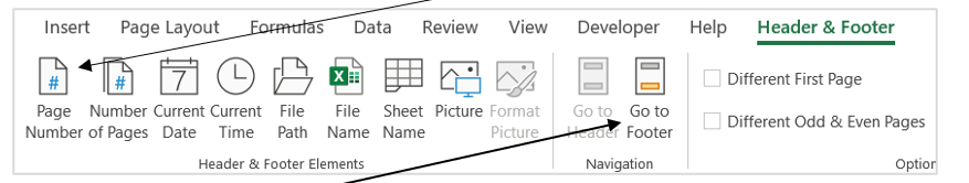
5. Click Go to Footer.
6. Click in the left section and then click File Name.
7. Click in the right section and type Last edited then press Spacebar once.
8. Click Current Date, press Spacebar and then click Current Time.
9. Click anywhere in the worksheet to exit from footer.
10. Save and close your workbook.
11. Upload the completed activity document to the TEP021 Activities folder on OneDrive.