Activity – Excel 6: Chart elements

[This section should take you around 30 minutes to complete]

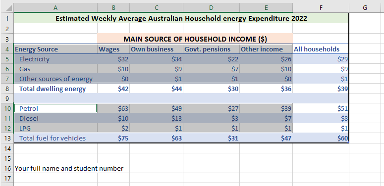
You will be using non-contiguous cell selection to create the chart that will compare the income with expenses in the table. When comparing data, total rows are not included. To compare the totals, a separate chart can be created that only includes that data.

1. Open your Activity 3 workbook and Save As Your Name TEP021 Excel 6 in the documents folder.
2. Delete the blank Column A.
3. Delete the blank Row 1.
4. Select the cell range A4:E7 and,
5. Hold down the Control key (<Ctrl>) and select the cell ranges A10:12 and,

Remember – Only plot the raw data on a chart. Totals and Averages should be plotted on a separate chart.

4. You should now see the following range of non-contiguous cells selected:

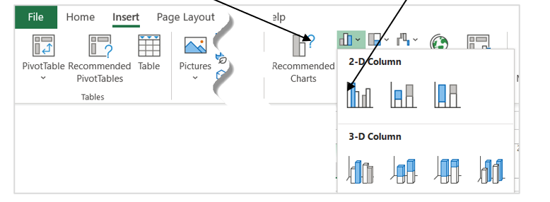
5. On the Insert ribbon, click the Column Chart icon and select Clustered Column.

6. Move the mouse pointer onto the outside border of the chart. When the mouse pointer changes to this icon, click and drag the chart below the data table.

Remember that a chart with no chart title and axis titles is meaningless. Readers can’t understand the content without the context that a title provides.

Adding Chart Elements

1. Click the Chart Elements icon and then tick the box for Axis Titles. You can add or remove chart elements by ticking or ticking off the boxes here.

2. The generic Chart Title, X-Axis Title, and Y-Axis Title are displayed on the chart.
3. Click Chart Title and then type Estimated Weekly Average Household Energy Expenditure 2012. The text appears in the Formula Bar only, the chart title is not yet updated.
4. Click anywhere outside of the textbox. The chart title is updated with the text just entered.
5. Click the horizontal Axis Title, type Energy Source, and press Enter key.
6. Click the vertical Axis Title, type Weekly Expense, and press Enter key.

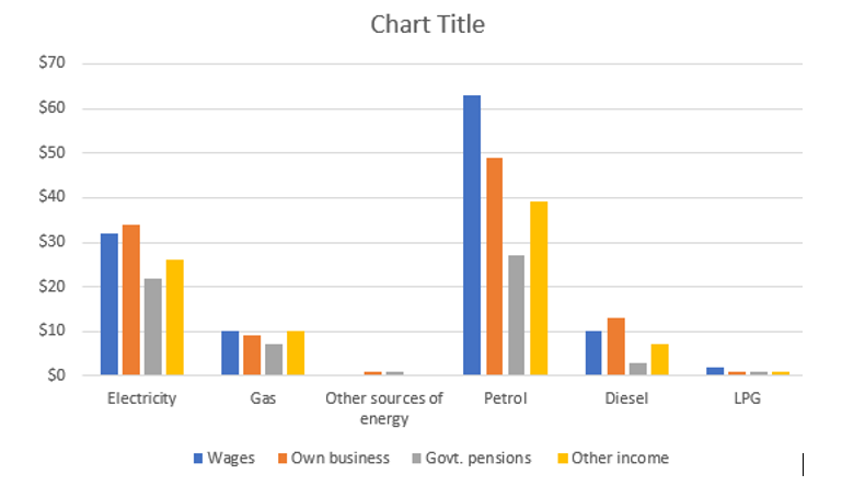
The chart should now look like this:

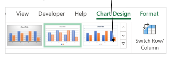
7. While the chart is still selected (active), click the More button of the Chart Styles (from the Chart design ribbon). Try each of the styles and then select one for your chart.

8. Click the Format tab.
   
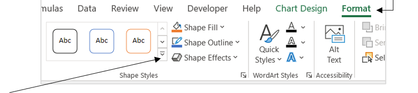
9. Click the More button on the Shape Styles. Try each of the styles and then select one for your chart.
10. Switch to the Page Layout view by clicking the Page Layout icon at the lower-right corner of the Excel window.

11. Check that the chart has not split across two pages. If it has, resize the chart by dragging the corners to fit it into the page OR drag the chart below the table.
12. Add a header with your name and student number on the left and the date on the right.
13. Add a footer with the unit code and activity name and number on the left, and a page number on the right.
14. Save and close your workbook.
15. Upload the completed activity document to the TEP021 Activities folder on OneDrive.