Activity – Excel 8: Inserting and moving data

1. Start a new Excel workbook.
2. Click the File tab and then Save As to save the spreadsheet as Your Name TEP021 Excel 8 in the Documents folder on your computer.
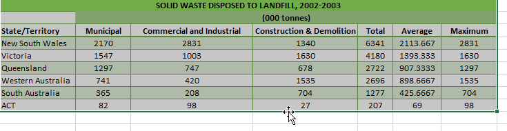
3. Enter the data as shown below.

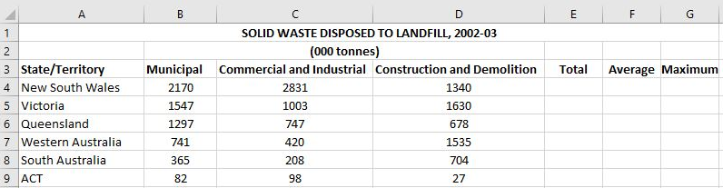
Source: Australian Bureau of Statistics, 2006.

4. Apply AutoFit Column Width so that your column sub-headings are visible.

5. Click A12 and type your full name and student number.

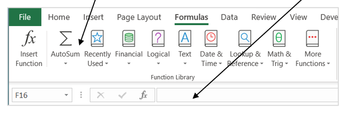
Inserting a Function using the AutoSum button

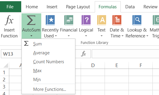
1. Click the Formulas tab
2. Click in cell E4.
3. Click the drop-down arrow for AutoSum
4. Click Sum.
5. Check to make sure the auto-selected data range is correct.
6. Press Enter key to complete the function.
7. Click (once only) back in cell E4 and AutoFill by dragging the Fill Handle down to E9.
8. Click in F4.
9. Click the drop-down arrow for AutoSum and select Average.

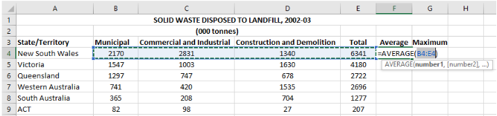
Notice that Excel picked up the data range B4:E4, all the numbers on the left; but E4 is the Total you just calculated, it’s not the original data. If you include the Total when you calculate the average, the result will not be correct.

Always check the computer-suggested data range in formulas and rectify if they are incorrect.

10. Change the data range B4:E4 to B4:D4 by doing one of the following:

• Click in B4 and drag to D4. OR
• Click in the Formula bar, delete E4 and then type D4 in.
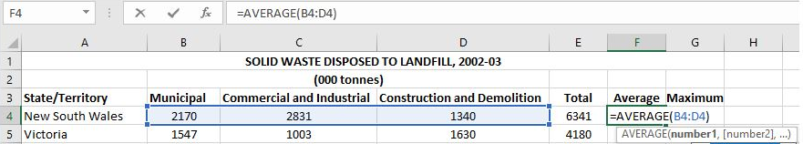
  11. Click the tick to complete your formula.
  12. AutoFill from F4 to F9.

Inserting a Function using the Function button (fx)

1. Click in cell G4.
2. Click the fx button in the Formulas tab OR the small fx button on the Formula bar.

Notice that the equal sign is automatically entered when clicking the fx icon and the Insert Function dialogue box is opened for you.

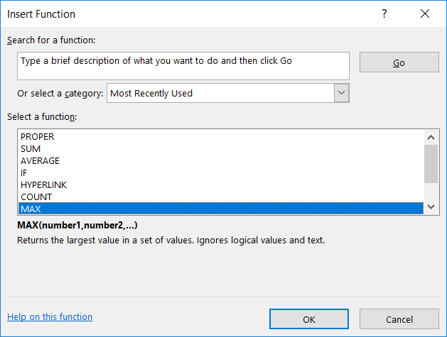
3. Click Max in the list to select it and then click OK.

Notice that Excel picked only one cell, F4, which is not correct. The correct data range should be B4:D4, the original data.

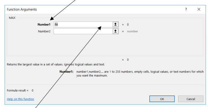
4. Click the Collapse button for Number 1.

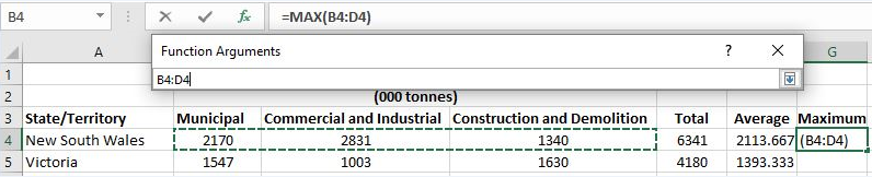
5. Change the data range B4:D4 by clicking in B4 and dragging it to D4.

6. Click the Expand button.

7. Click OK to complete the function.

8. AutoFill by dragging the Fill Handle down to G9.

9. Format the table title using the skills you learnt in the previous activity, such as Merge & Center, change font style, size and colour, fill background colour.

10. Apply a Table Style to the table (A3:G9).

11. Convert the table back to a data range to eliminate the buttons in the column headers.

12. Change the Page Layout Orientation to Landscape and make sure the table does not split across two pages

13. Select from cell B3 to G9 and apply Centre Alignment

14. Add a header with your name and student number on the left and the current date on the right.

15. Add a footer with the activity name and number on the left and page number on the right.

16. Save and close your workbook.

17. Upload the completed activity document to the TEP021 Activities folder on OneDrive.

Copying and Moving Data within Excel

When you need to copy or move data within Excel, you can use either Drag & Drop OR Copy and Paste.

Copying or Moving Data with Drag & Drop

1. Select the data range you want to copy or move.
2. 2. Move the mouse pointer over an edge of the selection so that the pointer turns to a move icon.

3. Click and drag the data to where you want it to appear and then release the mouse button. The selected data is moved to the new location.

If you want to copy the data rather than move it, hold the Ctrl key down and move the mouse pointer over an edge of the selection; when the mouse pointer turns to, drag the data to a new location.

Drag and drop moves or copies all of the data and all of its formatting.

Copying and Pasting with Options

Like Word and PowerPoint, you can copy and paste data to different locations within a worksheet, to a different worksheet, and even to a different workbook.

Excel provides more paste options than any other applications. With these options, you can choose to paste all or only part of the data you’ve copied, such as Values only or Formulas only.

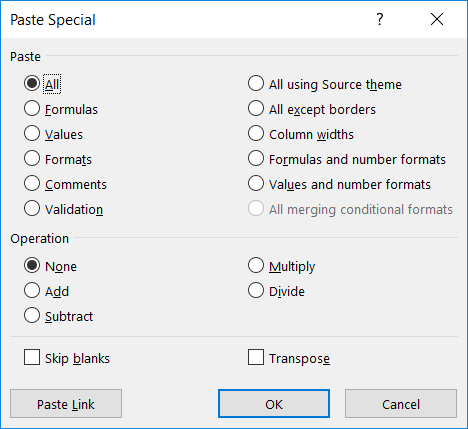
You can access even more options by clicking Paste Special…

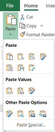
The list below explains what each option does.

There are a few more options not included in the Paste Options palette, but in the Paste Special dialogue box:

Comments. Select this option button to paste in only comments. This option is handy when you’re integrating different colleagues’ takes on the same worksheet.

Validation. Select this option button to paste in data-validation criteria.

Merge conditional formatting. Select this option button to copy all data and formatting and to merge in any conditional formatting.

Skip blanks. Select this check box to prevent Excel from pasting blank cells.